Share this blog:

Navigating Uniswap V2 With Volatility-Based Strategies
As decentralized finance (DeFi) participation increases, becoming a liquidity provider has emerged as a new way to generate yield or returns on decentralized exchanges and protocols.
A liquidity provider (LP) invests in crypto by staking their assets on a decentralized exchange (DEX) or protocol to earn a share of the pool’s transaction fees. The LP deposits an equivalent value of each underlying token in return for the pool tokens, which can be redeemed for the underlying assets at any time. This automated liquidity system replaces the traditional order book trade execution system with a liquidity pool of two assets that are valued relative to each other. As one asset is traded for another, the relative prices of the assets shift, determining a new market rate for both.

Uniswap is a decentralized exchange (DEX) that uses smart contracts on Ethereum to power its liquidity functions. Paired assets act as automated market makers (AMM), regulated by a constant product formula. In Uniswap Version 2 (v2), liquidity is evenly distributed, and liquidity providers only earn fees on a small portion of their capital. This may increase impermanent loss (IL) for LPs, and traders can be subject to high degrees of slippage as liquidity is spread more thinly over all price ranges.
In Uniswap Version 3 (v3), liquidity providers can concentrate their liquidity within a custom price range to maximize the use of their pooled assets. This gives individual LPs more control over where their capital is allocated and allows them to put far less capital at risk. For example, an liquidity provider in the USDC/ETH pool could allocate $1000 to the price range of $1500–2500 and another $500 to the price range of $2000–2250.
Factors Impacting Liquidity Providers
Successfully becoming a liquidity provider is not as simple as depositing assets into a pool and waiting to earn a profit. There are multiple factors to consider when deciding on which pair to provide liquidity for, such as the Total Value Locked (TVL) of a pair, the number of trades (trade volume) per day of the trading pair, and the characteristics and volatility of the particular asset. Additionally, the structure of determining fees and IL is complex and requires an in-depth analysis.
By using decentralized exchange and protocol data, we can equip ourselves with tools that allow us to dig deep into pool activity and help us make profitable investment decisions. In this research paper, we will first explore factors to consider when becoming a liquidity provider on Uniswap V2 by investigating the most popular liquidity pools. Next, we will take an in-depth look at how to calculate and evaluate fees and impermanent loss. Finally, we will leverage the Amberdata API to backtest LP rewards within different market conditions and discuss our findings. To view the code, please refer to our GitHub.
Uniswap Pool Statistics Analysis
Using the Amberdata Decentralized Exchange (DEX) API endpoints, we will first investigate the characteristics of four Uniswap v2 liquidity pools to understand their general behavior and performance. We split these four pools into two groups: DAI_ETH and ETH_USDC, and DAI_USDC and DAI_USDT. These two groups help us understand pool behavior and its characteristics by comparing each one to a similar baseline. With this, we can compare stablecoins to one another and stablecoins to ETH, as well as investigate the differences in transactions and APY.
First, let’s take a look at the Uniswap v2 DAI_ETH pool. DAI is a stablecoin made by MakerDAO whose value is pegged to the U.S. dollar. This is one of the most popular liquidity pools on Uni v2, and the Amberdata DeFi data allows us to break down the pool activity in four ways.
As shown in the Figure 1, the price of ETH fluctuates around 750 to 850 DAI. The total volume locked (TVL)
in the DAI_ETH pool has been hovering around 12-14M and has been decreasing slightly, while the volume has been volatile but overall decreasing. The number of trades has also decreased to under 200 a day, indicating that all pool movement is slowing.
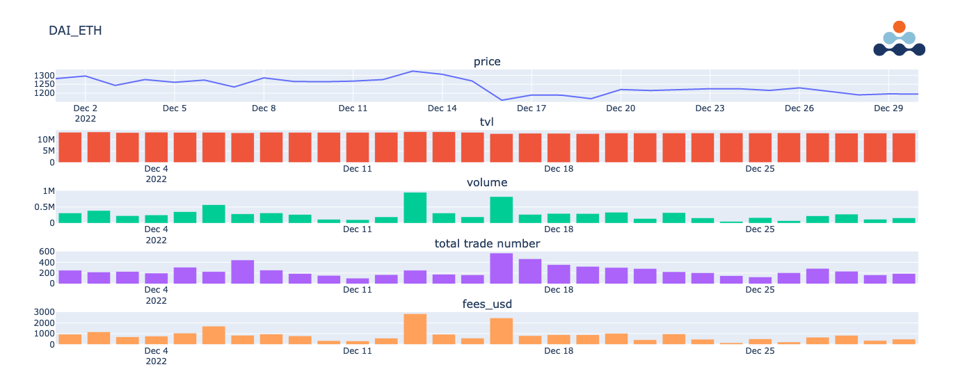
Figure 1 – The Uniswap v2 DAI_ETH Pool
The ETH_USDC pool, shown Figure 2, has similar patterns of total volume and trade numbers to the DAI_ETH pool. Both the TVL and volume remain around the same level but have been decreasing.
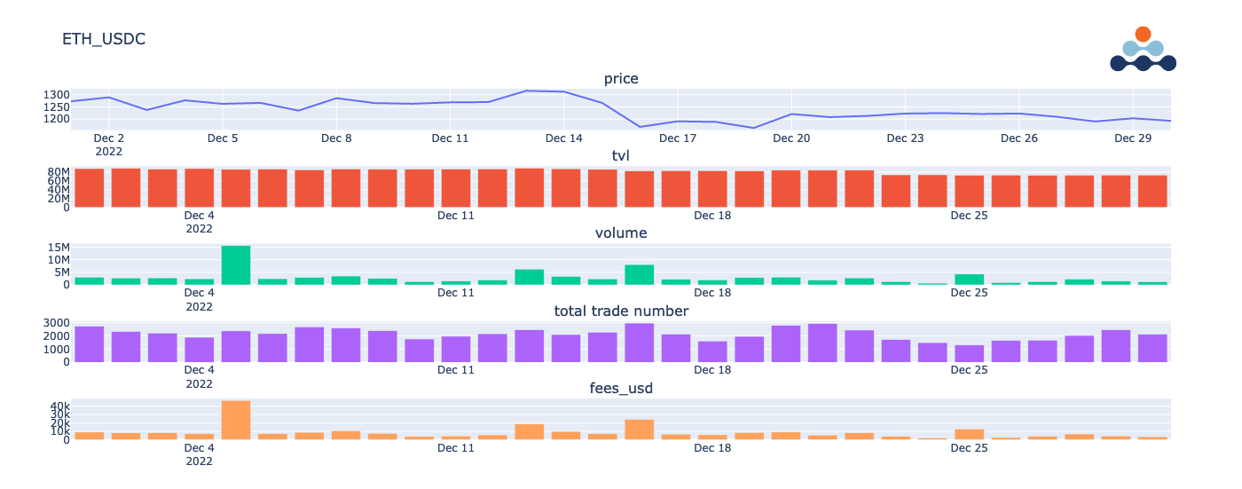
Figure 2 – The Uniswap v2 ETH_USDC Pool
To further compare these two pools, we will do a capital efficiency comparison by dividing the Volume by the TVL. For every event that occurs in a pool, liquidity providers share the trading profit of the total trade amount, which is 0.3% in Uniswap v2. Thus, the higher the trading volume per dollar amount in a pool, the higher profit an liquidity provider shares.
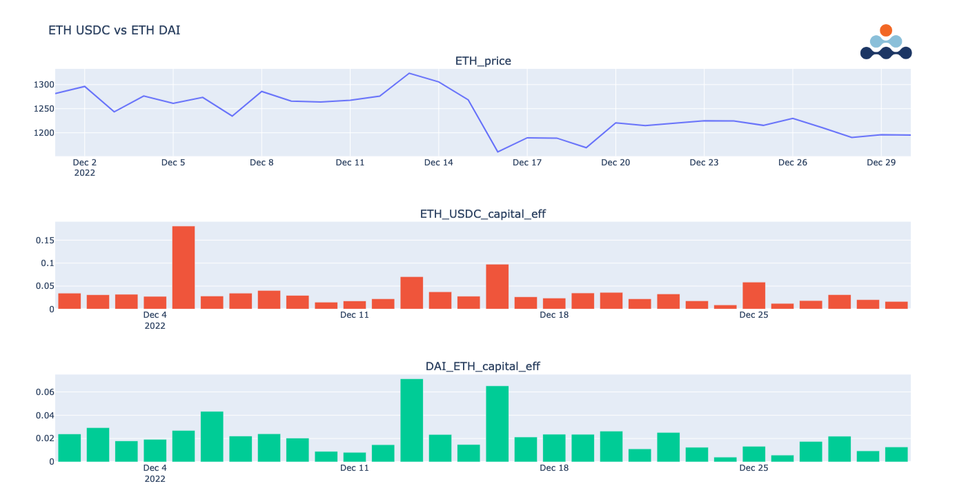
Figure 3 – Capital Efficiency Comparison for ETH_USDC vs ETH_DAI
Figure 3 illustrates how two liquidity pools that trade the same asset (ETH) can still have very different behaviors from each other. The ETH_USDC pool has higher capital efficiency metrics compared to the DAI_ETH pool. The ETH_USDC pool's capital efficiency is about twice as high as the DAI_ETH pool. Assuming all other conditions remain constant, this suggests that for each dollar invested in stablecoins as a liquidity provider, the ETH_USDC pool could generate approximately double the profits compared to the DAI_ETH pool. This analysis shows us that if a liquidity provider or trader is looking to deploy funds and if other conditions remain constant, the ETH_ USDC pool will likely make more profits.
Now, let’s look at our second pool comparison. In Figure 4, we can see that the DAI_USDC pool in Uniswap v2 has a lower trade volume and volume than other pools. These fluctuations and very low volumes on certain days could reflect current macroeconomic conditions.
Figure 4 – The Uniswap v2 DAI_USDC Pool
Finally, our DAI_USDT pool looks similar to the DAI_USDC pool but has a steady TVL at 6M.
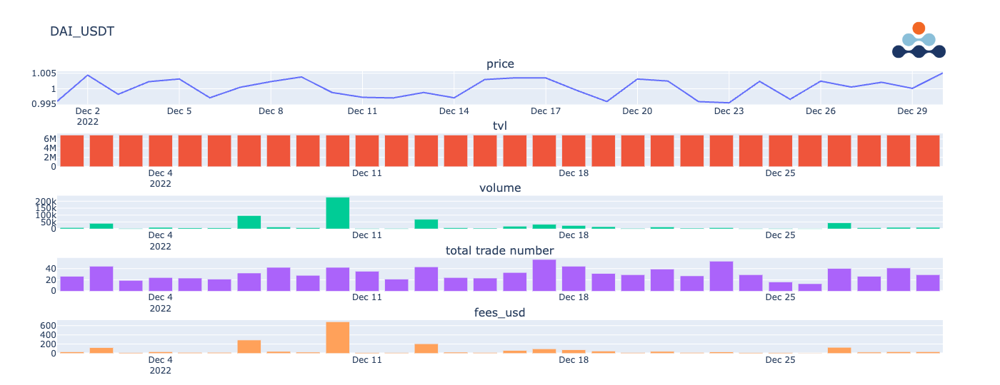
Figure 5 – The Uniswap v2 DAI_USDT Pool
If we compare the DAI_USDC and DAI_USDT pools in Uniswap v2 by dividing each pool’s volume over the total volume locked, we can show their capital efficiencies.
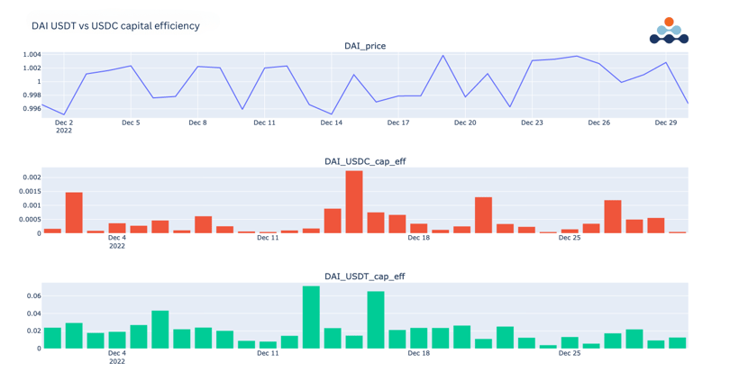
Figure 6 – Capital Efficiency Comparison for DAI USDT vs DAI USDC
When looking at these graphs, it is clear that the capital efficiency of the DAI_USDT pool is significantly higher than the DAI_USDC pool by an astonishing 400%. DAI and USDC are commonly used stablecoins in DeFi, but USDT is a less popular choice. It is therefore understandable that USDT liquidity providers have higher returns, as when fewer individuals provide funds to trade in the pool, there is a higher percentage of profits shared amongst liquidity providers.
We have only scratched the surface of liquidity pool behavior in Uniswap. The next two sections will dive into the structure of fees and impermanent loss.
Fee Analysis
Collecting percentages of liquidity pool fees is how liquidity providers earn a profit, but fees can be difficult to calculate. Since the fees collected when acting as a liquidity provider are calculated from what percentage of LP tokens you own compared to the total, users adding or removing liquidity changes the liquidity provider’s total ratio. To calculate the fee, it is necessary to not only track every swap amount but all liquidity events, adding a layer of difficulty to any backtested trading strategy.
Traditionally, there are different ways to calculate and backtest these fees, but we will explore one specific method that we used. Our approach involved using liquidity snapshots to track pool prices for every swap, mint, and burn event, combined with equations to calculate the total amounts of the trades. This is then simulated with the liquidity provider’s asset amount and the token ratio an LP provides is recalculated before and after all events mentioned above to obtain the fee.
Using the liquidity snapshot endpoints of the Amberdata API to calculate the liquidity provider fees collected simplifies the process of estimating our profit since we do not have to track LP tokens every single time a trade event happens. By simply tracking the pool’s price movements, we were able to automatically calculate the changes in our LP token ratios by using an equation, thus expediting the entire backtesting process.
Our Approach: Liquidity Snapshots
As a liquidity provider, your liquidity amount stays constant due to the automated market making constant product formula. Traders swap tokens (ex. USDC for ETH or vice versa) to move the prices up and down. Based on the direction of the swap, sometimes a trader will collect trading fees from USDC and sometimes from ETH. The fees collected can be calculated based on the before and after price of the pool’s token0 and token1.
Take Figure 7 below for example. Using the liquidity snapshot endpoints of the Amberdata API, we were able to show pool activity for every mint, swap, and burn event. A mint on Uniswap v2 refers to a user providing new liquidity into a pool. A swap refers to exchanging one cryptocurrency for the equivalent value of another, like one ETH for 2500 USDC. Depending on which asset is being swapped, (ex. ETH for USDC or USDC for ETH), the swap may raise or lower the price of the asset. A burn, similar to a stock buyback, is the process of taking tokens out of circulation. This reduces the total supply of the coin and may increase demand.
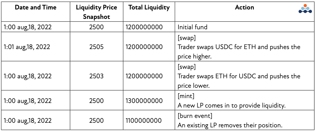
Figure 7 - Table showing liquidity price and total liquidity after pool events
The first swap of USDC for ETH in the pool raises the price of ETH from 2500 to 2505, while the second swap of ETH to USDC lowers the price of ETH to 2503. The mint event adds tokens to the pool, which lowers the price of ETH and increases the pool’s liquidity, and the burn event lowers the pool’s liquidity.
Every time the price goes up or down, the percentage of fees that an LP is earning in relation to the pool changes. Thus, we must use an equation to calculate the new liquidity and token prices.
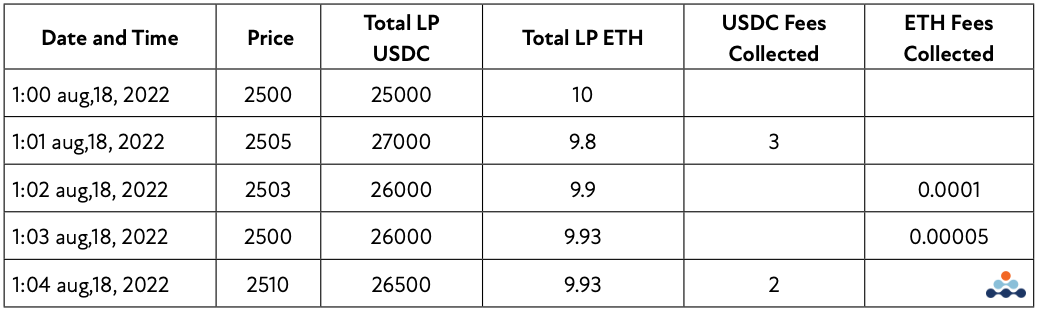
Figure 8 - Root table of Liquidity
As shown in Figure 8, if we use Amberdata’s liquidity snapshots for every swap, mint, and burn event, we can analyze all pool activity and simulate how much we can collect as a liquidity provider. By building the root table above and aggregating the fees from USDC and ETH separately, we can easily trace the total profit earned by the Liquidity Provider and use it to backtest our trading strategy.
Please skip to the appendix for an optional, in-depth analysis of calculating fees.
Impermanent Loss Analysis
Now that we are able to calculate the fees earned by a Liquidity Provider, we can explore another important factor of liquidity provider returns: Impermanent loss (IL). Impermanent loss is the opportunity cost a liquidity provider faces when a token’s price changes relative to its pair, between the time it is deposited in a liquidity pool and when it is withdrawn. The loss is considered impermanent because liquidity providers can recover their loss if the token pair returns to the initial exchange rate.
The bigger this change is, the more an LP is exposed to IL. This loss is referred to as impermanent because as long as your position is not closed out, the loss is not realized. Impermanent loss only affects profits when funds are removed from a pool, which means the timing itself hugely affects our total profit. For more information on impermanent loss, please read the Amberdata and Blockworks Investor’s Guide to Navigating Impermanent Loss.
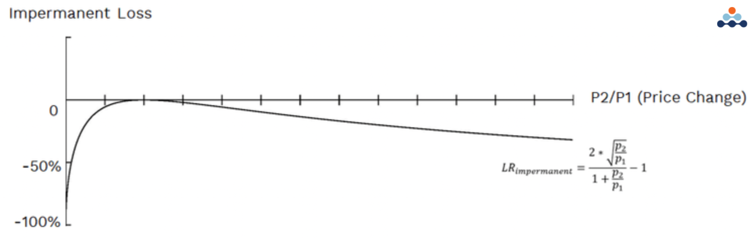
Let’s take a look at the mechanics of IL and how it fluctuates with price changes.
 Figure 9 - Position value after the initial price (P1) and the final price (P2) change
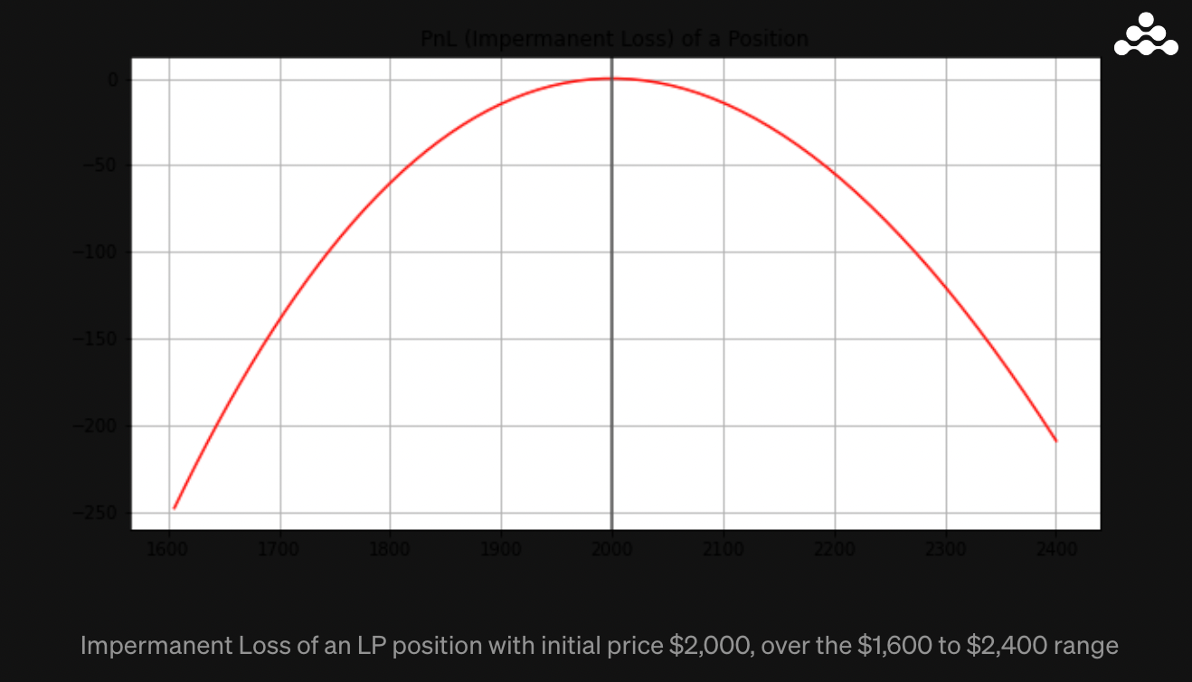
Figure 10 - Impermanent loss of an LP position equal to the change in price
Figure 9 showcases the position value after the initial price (P1) and the final price (P2) change. Figure 10 illustrates the same concept; as the value of the asset both decreases and increases, the IL is equal to the change in price. Whether the price change is negative or positive, there will still be IL, meaning the liquidity provider value will never be more than the original liquidity provided.
This is why understanding how to calculate fees and impermanent loss is so important. In order to generate capital as an LP, the profit earned from fees must be larger than the losses taken from IL.
Calculating impermanent loss is complex, but the core idea is simple and revolves around how the token ratios and values change while providing liquidity. When an LP deposits tokens in a pool to add liquidity, the ratio of fees earned will change.
Take Figure 11 for instance. Initially, there are 100 ETH and 40,000 DAI in the pool, but after a liquidity provider deposits their assets, the positions change to 105 ETH and 38,095.24 DAI. By recording every position’s change in prices (P1 and P2), we can calculate impermanent loss as the total value of ETH and DAI at T2 absent from the pool subtracted by the amount in the pool. In Figure 11, the IL would be $76.281-$76,190.48 = $90.52.
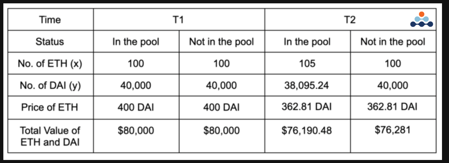
Figure 11 - Table illustrating ratio changes in a liquidity pool.
As mentioned previously, the appendix has an optional in-depth analysis of calculating fees and IL.
Backtesting Strategies: Providing Liquidity
Now that we have discussed the important elements of providing liquidity on Uniswap v2, it is time to deploy funds into our chosen pool to analyze its performance.
Using the DEX endpoints of the Amberdata API, we built a Python simulation framework to choose the most profitable pool based on TVL, Volume, Fees, and Impermanent Loss. We then analyzed all trade events within the pool to understand the total profit a liquidity provider would make.
Backtesting a liquidity-providing trading strategy helps investors understand profit and risks, profit and loss in varying market conditions, and the difference between the market price of a token and the profits from providing liquidity.
Backtested Performance Simulation Framework
After determining that the ETH_USDC pool was the most stable and lucrative pool on Uni v2, we first backtested our liquidity provider strategy against simply holding ETH and making a profit off of market-driven price increases. We call the simulation of holding only ETH a “full-holder,” and we use this as a benchmark for how our liquidity-providing strategy performs in comparison to how the price of ETH moves. We chose a wide period of time between March and June of 2022 so that we could investigate multiple different market conditions (rather than a more recent period, which would be primarily a downtrend).
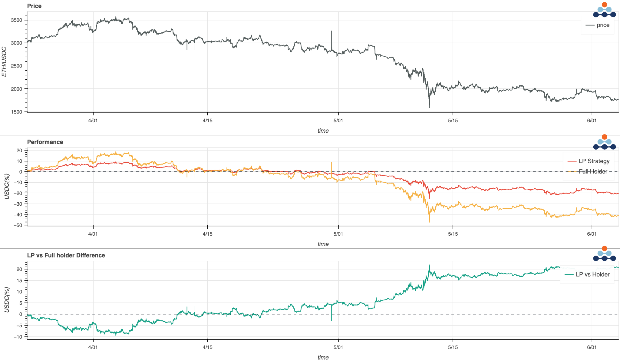
Figure 12 – Charts for analyzing LP performance against holding ETH
The first chart in Figure 12 illustrates the steady decline in the price of ETH in USDC from late March to early June of 2022. When we examine the second chart in Figure 12, we can see that our liquidity provider strategy had a more positive performance than if we were to use our fund to buy ETH and hold it in the allotted time. The third chart similarly illustrates the profit difference between a liquidity provider and an ETH holder. When the line is below zero, the ETH holder outperforms the liquidity provider, and when it is above zero, the liquidity provider outperformed the ETH holder.
While this is the first way many think to compare a liqudity provider strategy to the performance of a coin like ETH, this does not accurately represent the efficacy of providing liquidity. To provide liquidity in a pool on Uni v2, a token holder must split their tokens 50/50 - in this case, into half ETH and half USDC. Because of this, it is most accurate to compare liquidity provider returns to a simulated half-holder, or someone who holds an even split of ETH and USDC.
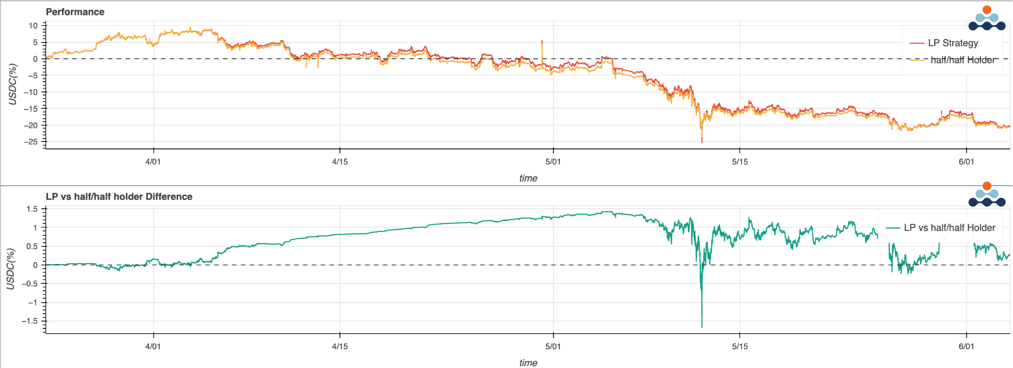
Figure 13 - Backtested performance of LP strategy half/half holder
The first chart in Figure 13 shows the backtested performance of our liquidity provider strategy, which requires funds to be split into half ETH and half USDC, compared to if we had held onto half ETH and half USDC. The liquidity provider performance is composed of the asset itself as well as fee collections within the pool. The second chart in Figure 13 illustrates the difference in the liquidity provider strategy from the half/half holder and shows that the LP is usually outperforming the half holder.
Providing Liquidity in Varying Market Conditions
Now, we will explore how profits earned from providing liquidity may shift and vary with macroeconomic conditions.
Uptrend Market Analysis
From mid-March to mid-April of 2022, ETH slowly increased in value from around $3000 to $3400.
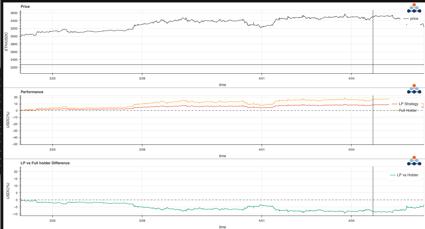
Figure 14 - Backtested performance of our LP strategy
As we can see from the charts in Figure 14 above, as the ETH price slowly goes up, the full-hand holder outperformed the liquidity provider. As the price of ETH increases, the liquidity provider’s ETH position is gradually being swapped for USDC, diminishing its potential profitability. As also shown in Figure 14, when ETH prices rise about 10%, the LP’s profit only increases by 5% - around half of the full-holder’s profits. This is due to the structure of Uni v2, where half of the LP’s fund is invested in USDC rather than only ETH.
In order to quantify the impact of the pool’s swap events, we must exclude the impact of half of the LP’s assets being invested in USDC. To understand exactly how providing liquidity impacts our profits, we compared our liquidity provider strategy to a holder with half USDC and half ETH to mimic the liquidity provider’s assets.
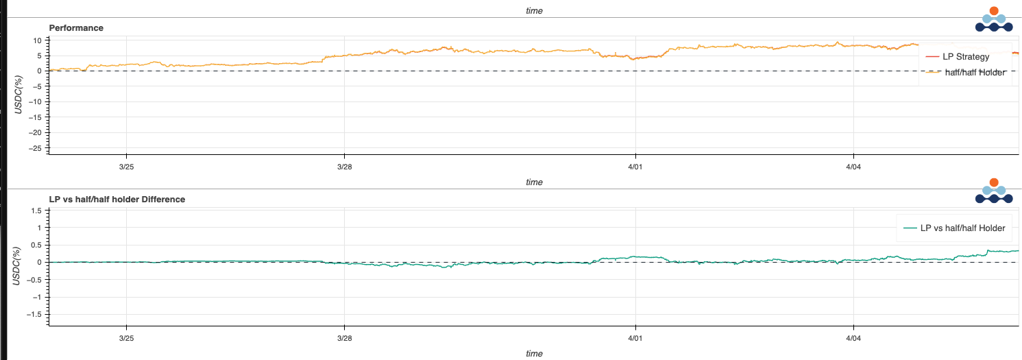
Figure 15 - Liquidity provider strategy vs. a holder with half USDC and half ETH
The green line in the second chart of Figure 15 above shows the profit difference between our liquidity provider strategy and a holder of half USDC and half ETH. With the same slow uptrend market conditions as the full holder graphs, we can observe that there are no significant differences between investing funds into a Uni v2 pool versus holding ETH and USDC. This indicates that there is no potential alpha to be earned under slow uptrend market conditions.
Downtrend Market Analysis
Now, let’s take a look at how our LP strategy performs in downtrend market conditions. Within a two-month test period, the price of ETH dropped 33% from 3,000 USDC to 2,000 USDC.
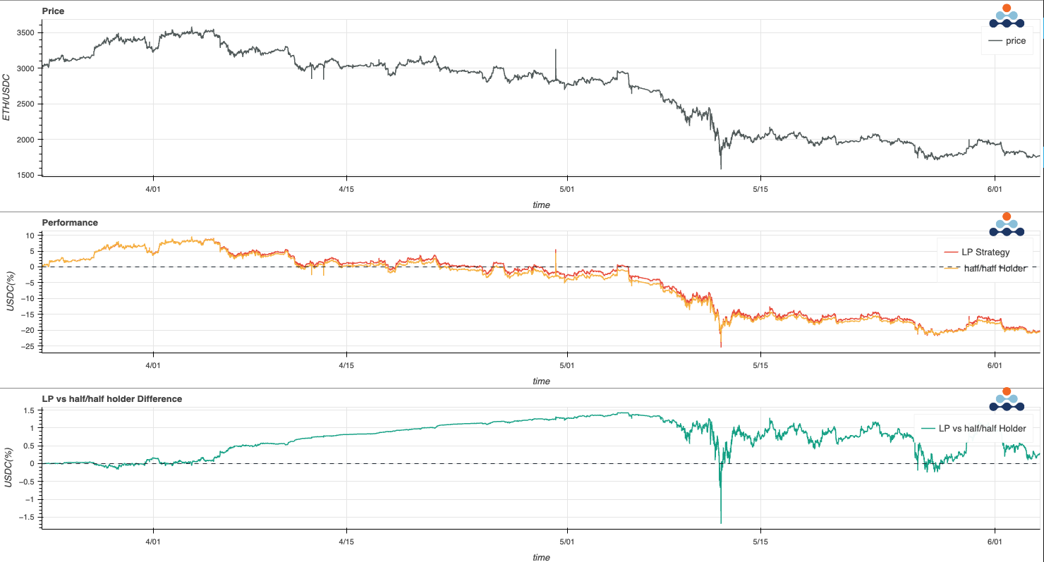
Figure 16 - LP strategy performance in downtrend market conditions
If we look at the difference between our LP strategy and a half-holder in Figure 16, we can see that out of the sixty-day test period, our LP strategy performed 0.5–1% better than the half-holder 95% of the time. When the liquidity provider strategy does worse than the half-holder, it is due to extreme market conditions and bounces back once the market has stabilized slightly. Overall, the liquidity provider strategy performs better than holding tokens in most downtrend market conditions.
Volatile Market Analysis
We have already learned that uptrend market conditions do not have a large impact on LP profits, but what about when the market is volatile? We chose a period of two days, 1/20-1/22, where the price of ETH dropped dramatically from 3200 USDC to 2400 USDC - a 25% loss.
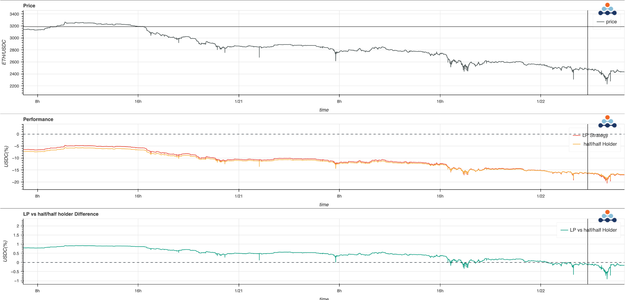
Figure 17 - LP strategy performance in volatile market conditions
While this steep drop in the price of ETH negatively affected our profit, it was not as impactful as one might think. In a worst-case scenario like this, providing liquidity has nearly the same effect as being a half- holder. Additionally, the price of ETH increased after these two days, emphasizing that certain losses may be impermanent.
Choppy Market Analysis
Choppy market conditions refer to when the market frequently swings up and down with volatility but has no apparent trend. As you can see from Figure 18, although the price of ETH is increasing and decreasing, its overall movement is oscillating around $3k.
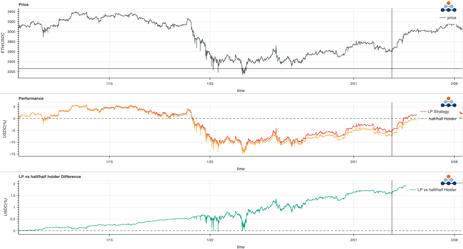
Figure 18 - LP strategy performance in choppy market conditions
Focusing on the third chart in Figure 18, where the green line indicates the difference between our LP strategy and a half holder, we can see that when the ETH price oscillates around $3,000, the liquidity provider outperformed the holder by about 2%! The combination of providing liquidity and collecting fees while minimizing IL creates the largest profit and highlights the benefit of being an LP when the market is choppy.
ppy.
In our last DeFi research paper, we discussed arbitrage between decentralized and centralized exchanges and how volatile market conditions make for optimal arbitrage scenarios. It is clear that volatility can bring huge benefits to traders who understand how to properly analyze market conditions.
Backtesting Summary
We now have tested multiple market scenarios including upward trend, downward trend, volatile, and choppy market conditions. Here is a summary of what we have found:
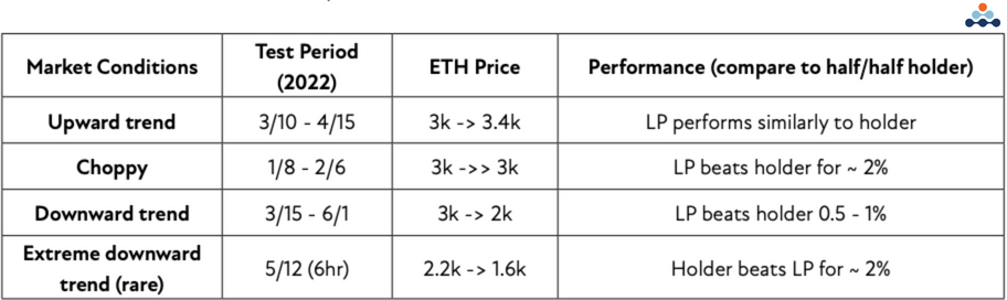
Figure 19 – Summary of LP strategy performance in different market conditions
Although a common perception is that providing liquidity during upward trending markets is not as profitable as holding the assets, our backtesting results show that there is no strong difference between the two.
In fact, in every scenario but extremely downward trending markets, our liquidity provider strategy performed better than a holder of half ETH and half USDC. Additionally, when the market is steady and shows no trend, liquidity providers have profits about 2% higher than the holder since a percentage of trading fees are being collected and there is little to no impermanent loss.
During a slow-moving downtrend market when all profits are decreasing, liquidity providers and half-holders still have similar performances. However, when the market plummets rapidly, our LP profits decreased, and our strategy performed worse. When bear markets like this emerge, it is important to close out LP positions fast as the resulting impermanent loss would heavily impact returns.
Overall, providing liquidity requires patience and trust that the market (and returns) will recover once volatility is back within a reasonable range.
Conclusion
In this research paper, we have discussed the factors to consider when picking a pool on Uni v2, such as the total value locked (TVL) of a pair, the number of trades (trade volume) per day of the pair, and the characteristics and volatility of the asset itself. After comparing a few Uni v2 liquidity pools, we examined the structure of liquidity provider fees and impermanent loss and how the two interact with one another. We then backtested a trading strategy on the ETH_USDC pool and examined our LP performance in varying market conditions. Our code can be viewed here.
Our final takeaway is that providing liquidity on Uniswap v2 may be a profitable strategy for those who are looking for a safer way to hold crypto assets. Liquidity provider strategies perform well in choppy market conditions and do not have significant differences from holding the assets during upward and downward trends.
Amberdata has full liquidity snapshots for decentralized exchanges like Uniswap. We also offer Uniswap v2 and v3 DEX data that shows movement from the wallet, pool, and protocol levels of the exchange. You can leverage Amberdata's DeFi offerings to track liquidity providers, identify patterns and trends for specific pools, mitigate risk, and generate profits.
Citations:
-
https://blog.amberdata.io/the-investors-guide-to-navigating-impermanent-loss
-
https://blockworks.co/the-investors-guide-to-navigating-impermanent-loss/
- https://github.com/amberdata
DISCLAIMER: The information provided in this research is for educational purposes only and is not investment or financial advice. Please do your own research before making any investment decisions. None of the information in this report constitutes, or should be relied on as, a suggestion, offer, or other solicitation to engage in, or refrain from engaging in, any purchase, sale, or any other any investment-related activity. Cryptocurrency investments are volatile and high risk in nature. Don't invest more than what you can afford to lose.
Appendix: Fee and Impermanent Loss Calculations
Fee calculation
Let’s dive deeper into how to calculate liquidity and price. The Uniswap automated market making (AMM) function is represented in the equation X*Y = K, where X denotes the total USDC amount a single LP provides, Y represents the total ETH amount a single LP provides, and k represents liquidity.
When the price of ETH is at 2500 USDC, assume a trader provides liquidity with 10 ETH and 25000 USDC. Uniswap requires liquidity providers to provide liquidity at a 50/50 ratio, meaning that our total liquidity is 10 ETH * 25000 USDC = k = 250000.
Based on our equation, if the pool price = 2500, we can write these equations.
Equation A: X * Y = 250000 = k = liquidity
Equation B (price): X / Y = N = 2500 = USDC per ETH
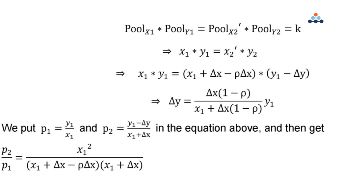
At the new pool price after a swap event, shown in Figure 2.3.1, we can also write that:
Equation C: X' * Y' = 250000 = K = liquidity
Equation D (price): X' / Y' = N' = 2505 = USDC per ETH
The total liquidity a single LP provides should remain constant. Thus, by using the equations above we can derive X' and Y', which represent the new total amount of USDC and ETH we have provided. After additional calculations, we can rearrange these equations to represent the new amounts:
X' = N' * Y' = new USDC amount
Y' = √( K / N') = new ETH amount
Now, to calculate the fees. Fees collected as an liquidity provider can be represented in the following equation:
Fees = (New USDC amount - Previous USDC amount) * (fee_tier/(1-fee_tier) ).
Fee tiers represent 0.3% for a liquidity provider on Uni v2.
Impermanent loss calculation and chart
Here is a mathematical proof of how to use the equation to draw the impermanent loss chart with respect to price change.
After these calculations, we can obtain the following equation, where p1 = initial asset price and p2= final asset price.
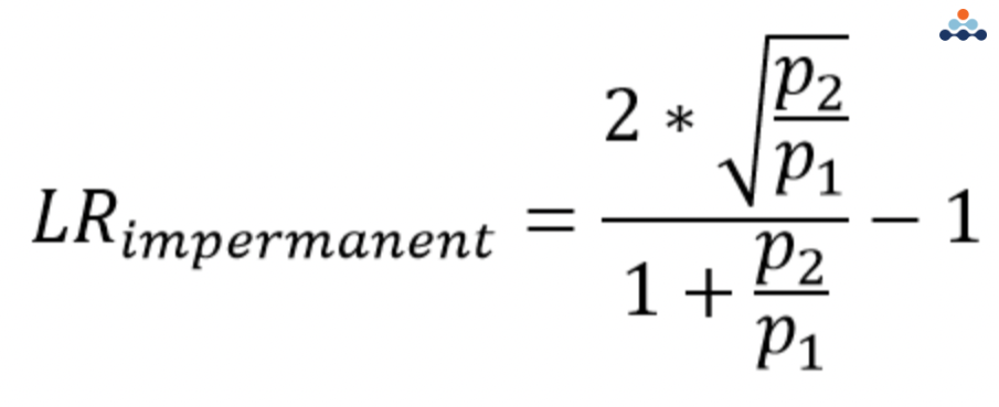
Thus, by using the liquidity provider metric, we can see how price changes affect our total position value. We learn that no matter how the price movement is, we will always have IL loss. The most important part is how can fee compensate our loss so we can gain profit in the end.