Simple Portfolio Optimization with Monte Carlo Analysis

Cryptocurrencies are evolving into a new asset class which is attracting the attention of many investors. Digital assets are radically transparent once you have access to the data. You will be relieved to know that much of what you know about traditional financial markets apply.

This is the second post of the series. You can read the first here to get set up, download some data and do some basic analysis of risk-adjusted returns using Sharpe Ratios on Cryptocurrency market data from the Coinbase Exchange.

Through this series of posts, we plan to show you how to gain access to the data and apply financial fundamentals to quantify opportunity, manage risk and hopefully create some Alpha. In this post, we will build a portfolio of the 10 most liquid assets on Coinbase then do some simple portfolio optimization via Monte Carlo Analysis.

I work at Amberdata so we are going to use our APIs. Amberdata solves a fundamental data infrastructure problem for anyone building on blockchain or transacting in digital assets. You will need an API key to code along with us during this series of posts. To get started sign up for the OnDemand plan. Download the Jupyter Notebook here

Let’s get some data. We are going to use Python, Jupyter Notebook and Amberdata’s API docs.

Let’s make it easy to read in any historical market data we want to look at. You will need to replace “YOUR_API_KEY” with your API key in the headers section so you can get access to the data.

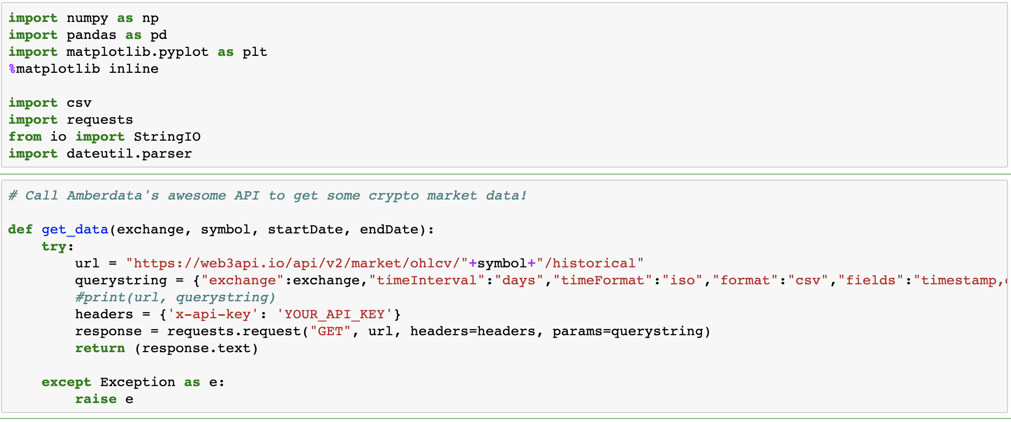
Here we call the get historical Open, High, Low, Close, Volume Endpoint as follows to pull in CoinbasePro historical data from Amberdata for the digital assets we are interested in.

Look at Analysis of Digital Assets for fun and profits with the Amberdata API and Jupyter Notebook #1 for the details on getting started.

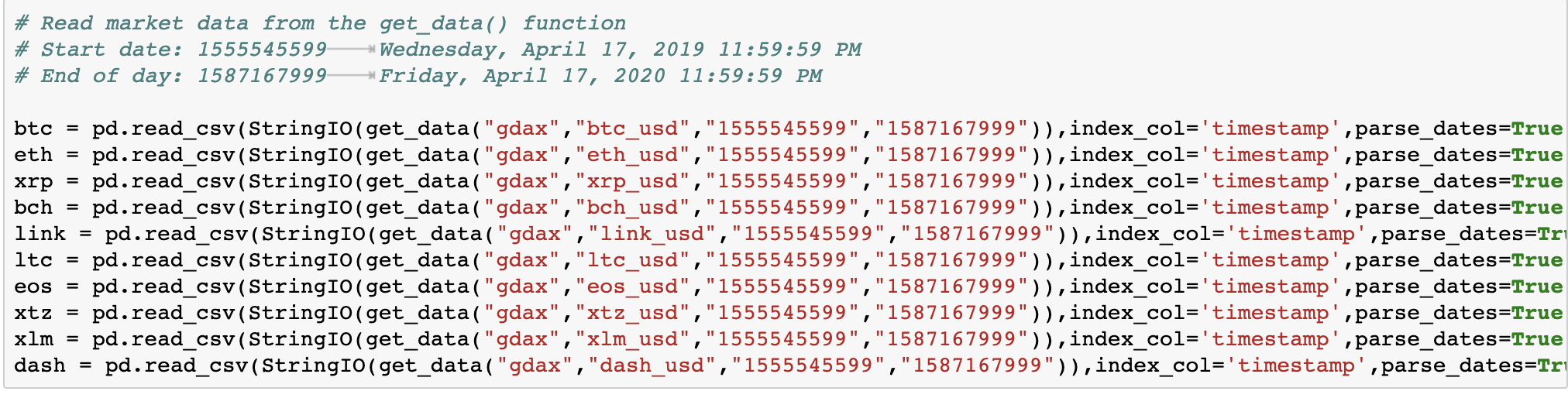
We are going to look at a year of data for the same 10 digital assets as in the last post. We simply sorted assets by liquid market cap which trade on CoinbasePro and that are USD denominated pairs so we don’t have to deal with cross-exchange or cross-rates.

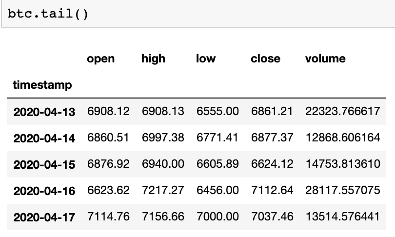
Let’s check to see that we have some data.

Now let's create a portfolio of digital assets. Since the digital asset markets never officially close. We have used the last minute of the day in GMT to represent the close 11:59:59 PM.

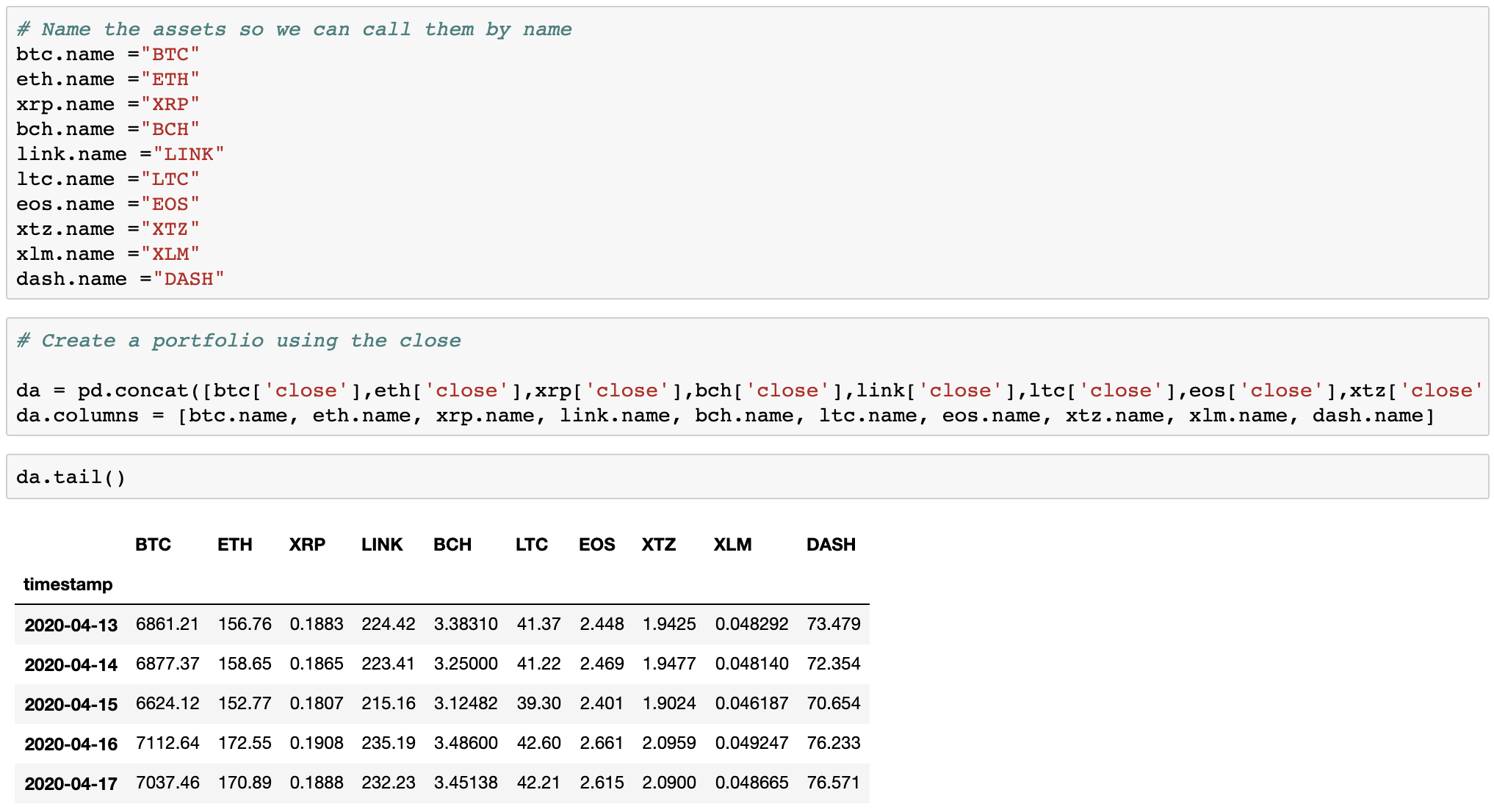
We can take a quick look at how these assets have performed by normalizing price activity and creating a time series simply by dividing daily close by the initial close.

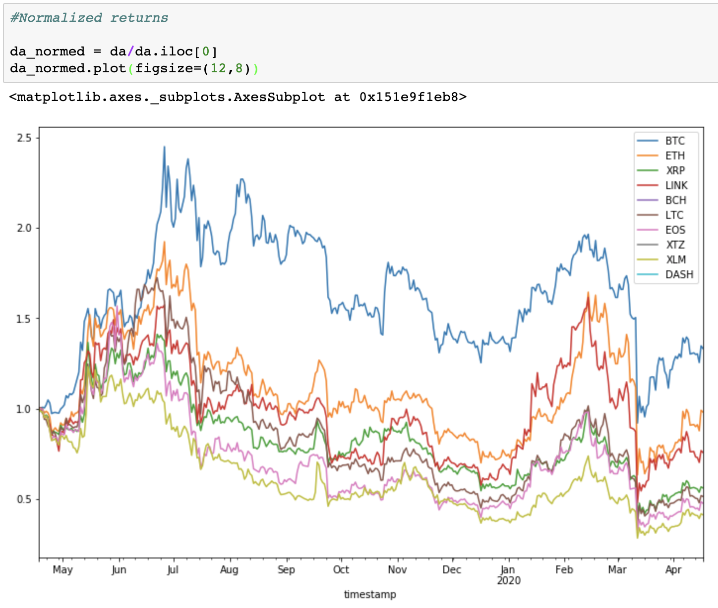
A quick look at the normalized returns implies that these assets may move together. How correlated are they?

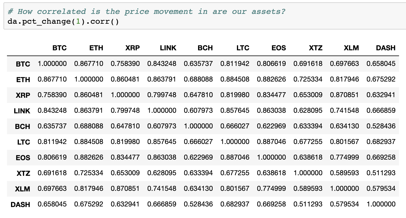
The data shows a positive correlation in fact. Where +1 assets should move in tandem and -1 inversely. The majority of these assets gains appear to be ~75% correlated with btc_usd.

Now let's calculate the log normal returns to de-trend the data.

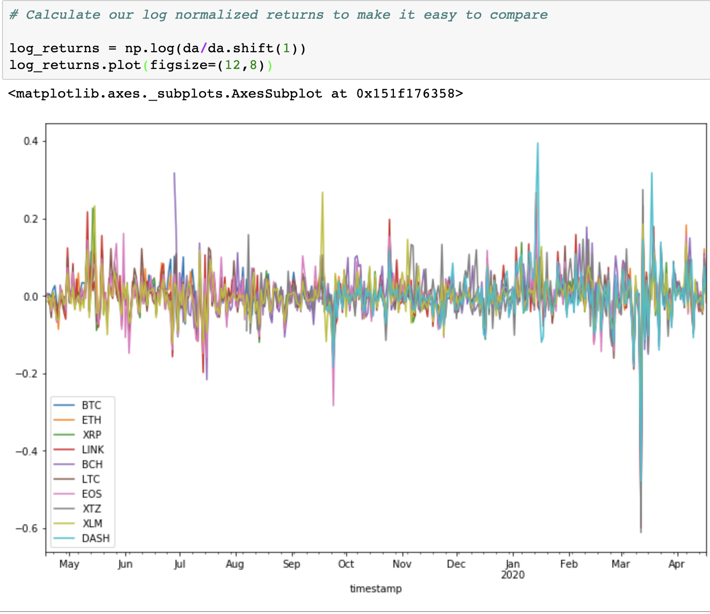
It looks like digital assets can be pretty volatile.

What were the risk-adjusted returns as measured by Sharpe Ratio on our base portfolio with equally allocated position sizes?

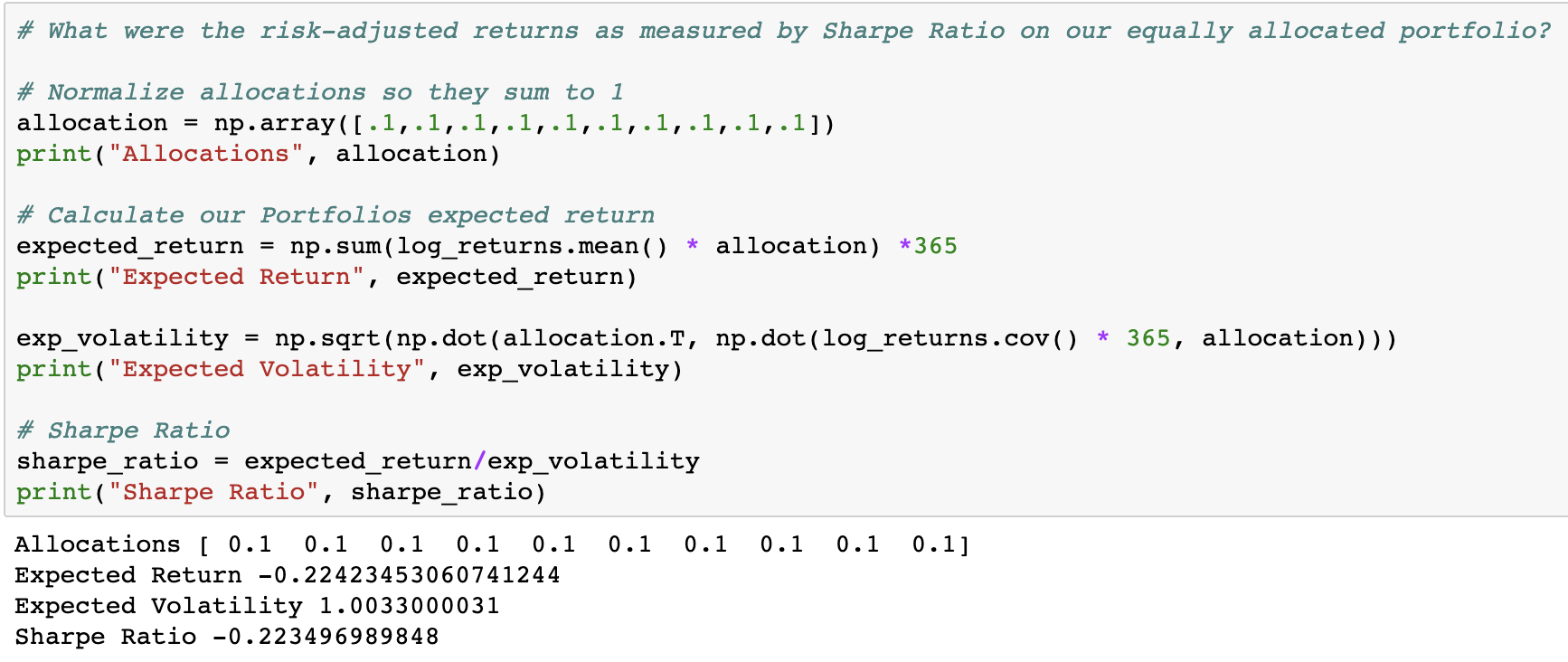
Here we can see that just holding an equally weighted portfolio of these assets for this time period may not be a good investment strategy as the portfolio is showing a negative expected return. The Shape ratio is also negative which means that the expected performance is below the risk-free rate which is zero today.

Can we MPT to optimize the portfolio and improve our expected returns? Let's use a basic Monte Carlo Simulation to find the optimal portfolio allocations. Obviously we are starting with a losing portfolio so let's see if we can improve the expected returns on a risk-adjusted basis via our portfolio allocations.

We have 10 assets in our portfolio, so we are going to generate 10 random numbers, normalize the sum of those to equal 1 and then calculate the expected return, expected volatility and Sharpe ratio for that portfolio as allocated.

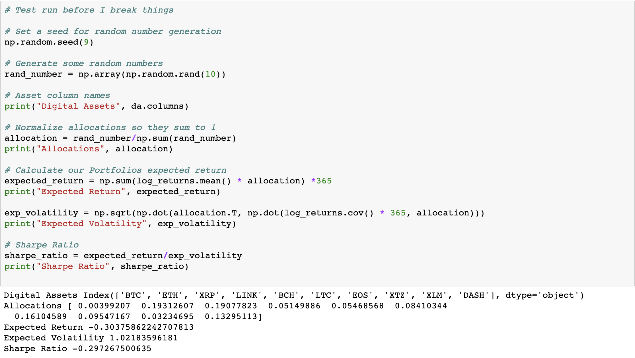
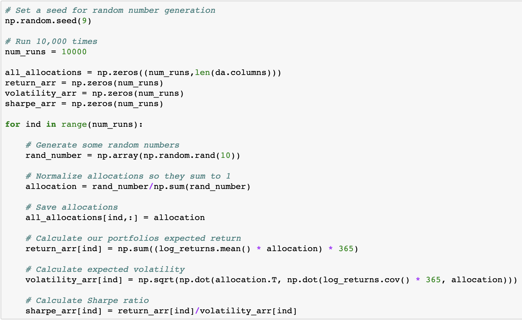
Our single pass test run actually performed worse than our portfolio so that's always fun. Let's run this 10,000 times and see if we can find the optimal allocations.

Our results show that we improved our Sharpe ratio from -.223 to .154 which is a lot better but still not compelling as a buy and hold portfolio.

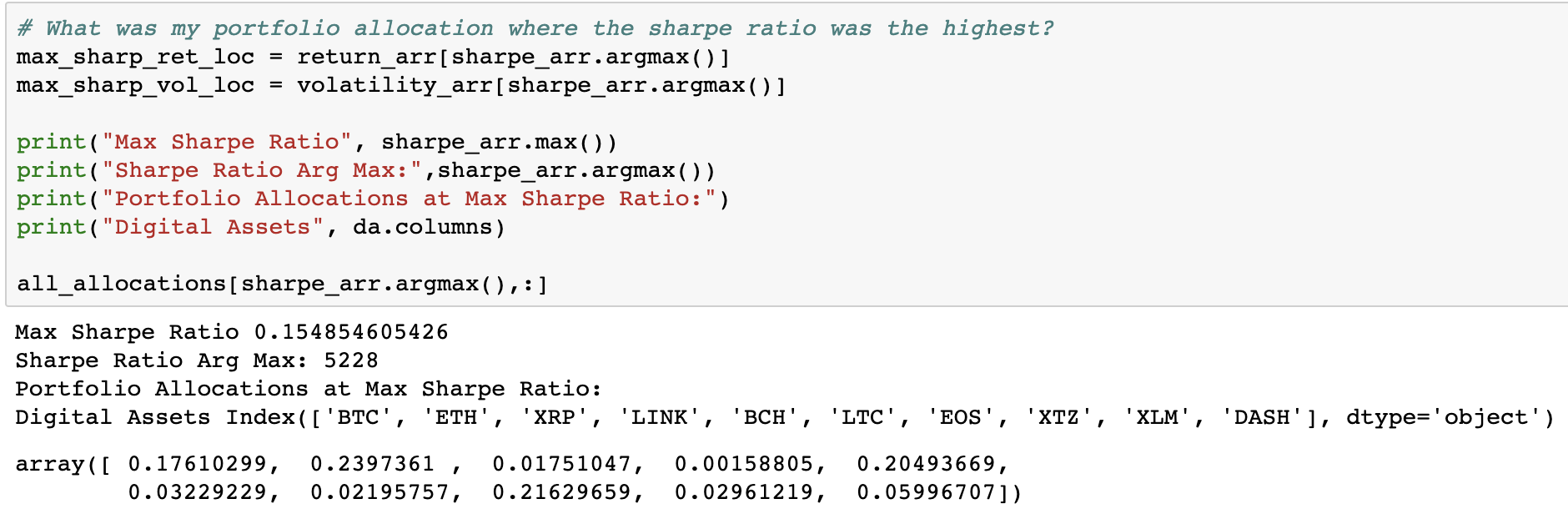
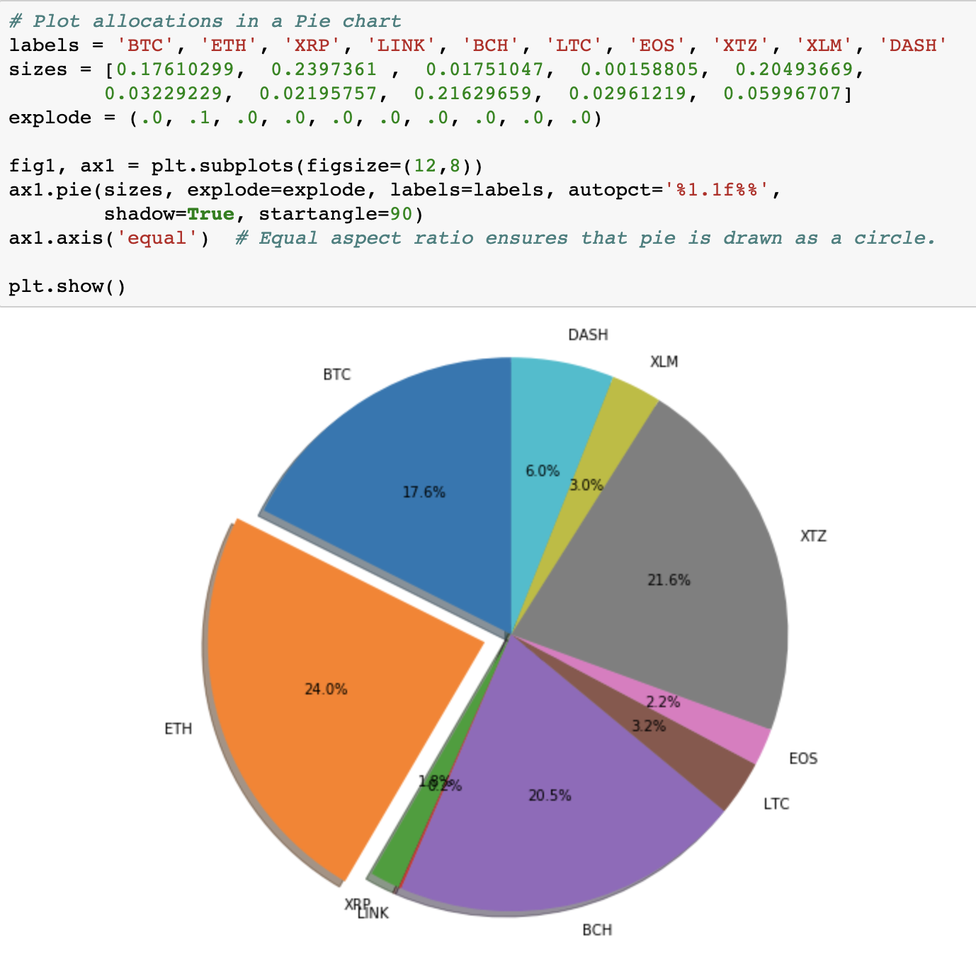
The best allocation after 10,000 runs weighted ETH, XTZ, BCH, and BTC more heavily.

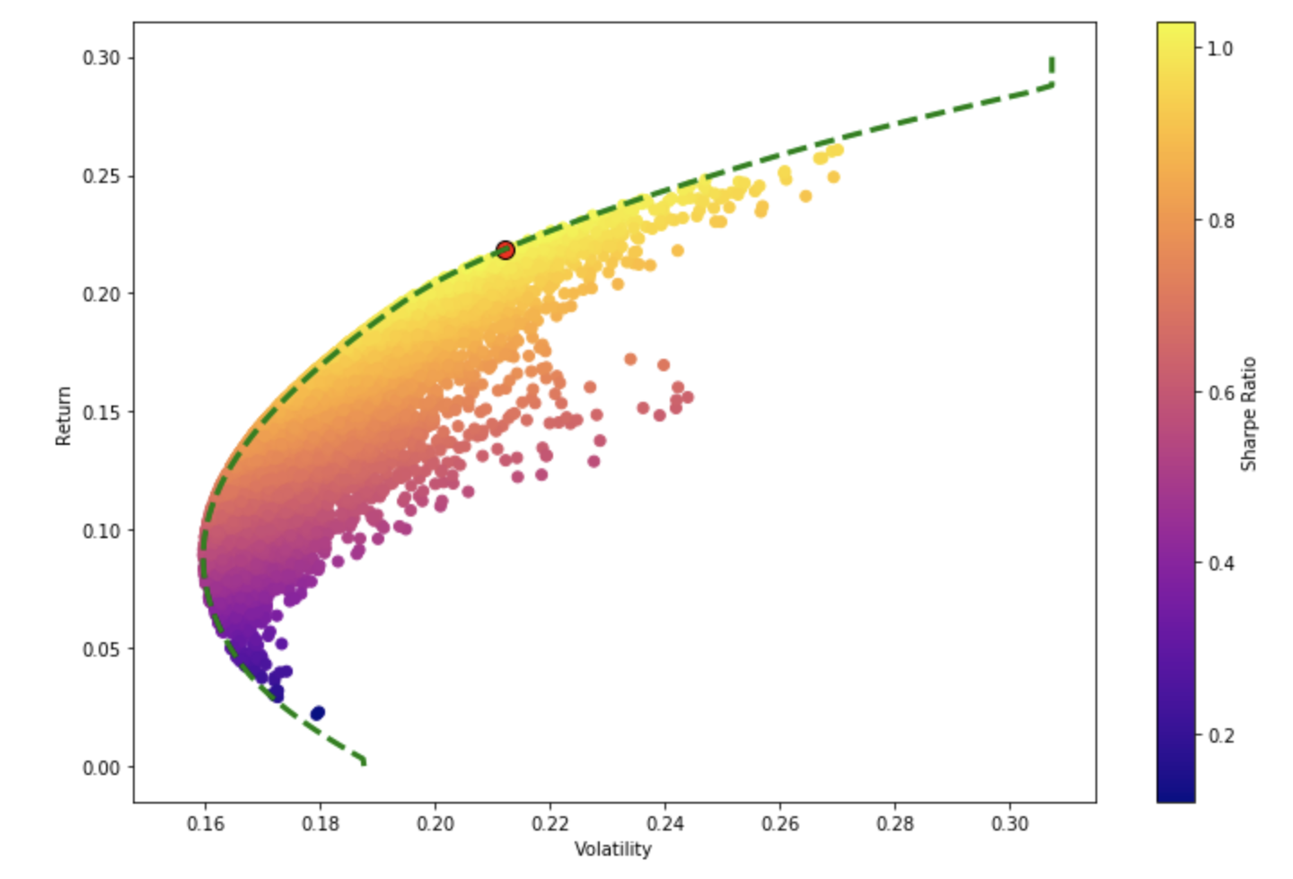
Unfortunately, our portfolio was a bit too volatile to generate an Efficient Frontier. We had hoped our plot would look like this.

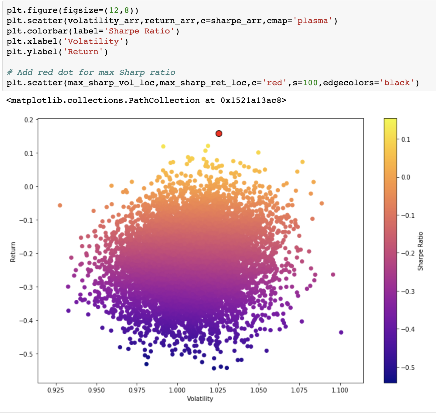
But we ended up optimizing to an outlier generated by our Monte Carlo simulation.

In this post, we pulled in a year of historical market data from the Amberdata API, quantified the risk-adjusted returns of that portfolio and then applied modern portfolio theory seeking the optimal allocation generated by a Monte Carlo analysis. In future posts, we will develop trading and money management strategies leveraging market and on-chain data to generate some Alpha.

Signup for our API and watch for our next post to help you unlock digital assets data. Download the Jupyter Notebook here

I want to give a shout out to the Python for Financial Analysis and Algorithmic Trading Course by Jose Portilla as I’ve pulled from some of his work here.