September 3, 2020

Bitcoin Sharpe Ratio: The Risk And Reward of Investing In Cryptocurrencies

Applying the financial meter stick for evaluating risk-adjusted returns of a (digital) asset, portfolio, or strategy.

People like to imagine that investors just care about how much money they make at the end of the day, but often forget that how the money is made matters as well.

While Pablo Escobar made it onto a 1989 Forbes article of wealthiest billionaires alongside Sam Walton — the founder of Walmart, nobody would confuse the way they made their fortunes. One passed on their wealth and created one of America’s wealthiest dynasties, while the other was shot and killed by Columbian authorities.

What does this have to do with investing, you may ask? Well, consider that making a 10% return on stocks is common while it would be nearly unheard of in bonds, for example.

This has to do with the fact that bonds are often less risky if held to maturity as an investment than equities. In other words, how risky an investment is matters as well as how big the returns are at the end of the day.

The Sharpe ratio takes this into consideration, and is an important metric for evaluating the performance of assets or a portfolio. This metric provides a standardized way of measuring how well your investments or strategies are performing, and how it does so is simple to understand.

First, we will go into detail about the Sharpe ratio and how it is used, and then we will combine data from sources such as Yahoo Finance for daily OHLCV asset data, and Amberdata for digital asset prices and metrics to investigate the Sharpe ratio — or risk-adjusted returns — of some popular assets such as gold and cryptocurrency.

Motivation

Let us say that you have created a portfolio that returns you 10% per year, net of expenses. That may seem great on the surface, but there are more questions that need to be answered first.

First, what is the risk profile of the portfolio? Are they in real-estate, small-cap stocks, commodities, large-cap stocks, equity, options, bonds, or some combination of the above? An 8% return on bonds would be incredible, but lackluster in small-cap stocks when you could just invest in a broad index fund and likely achieve better returns.

Second, how consistent are your returns? If you can beat the market by 25% one year, but you lose -15% on the market next year, then the portfolio is not very consistent and you may consider finding a more reliable investment despite the promising returns on year one.

The Sharpe ratio combines this information and addresses the need to evaluate the performance of an asset or strategy. It is not the only metric to look at when measuring performance, but it is the most widely used and often first quoted number.

In short, it is a measure of the quality of returns, which is why it is called risk-adjusted returns. Before we get into how it is calculated and use it in practice, we must talk about the Sharpe ratio’s lesser-known variant — the Information ratio.

Information Ratio

You will be glad to know that everything I said above is actually a lie. We will refer to the metric that incorporates all of the information above as the Information ratio. According to Investopedia, the Information ratio is defined as the portfolio return minus benchmark return divided by the tracking error. In other words:

IR = (Portfolio Returns — Benchmark Returns)/Tracking Error,

where the tracking error is the standard deviation of the difference between portfolio returns and benchmark returns. Ernest Chan has a little bit cleaner of a definition in his book Quantitative Trading, where he defines the information ratio as such:

Information Ratio = Excess Returns/Standard Deviation of Excess Returns,

where excess returns are the portfolio returns minus the benchmark returns. While articles such as the Investopedia article describe how to calculate the ratio, the key with using it effectively is to choose the right benchmark.

For example, if we are trading large-cap stocks, then the benchmark would be the S&P 500. Likewise, if we were trading gold futures, then the market index should be the gold spot price. In any case we choose the most similar and the most widely used asset in the same asset class as the benchmark.

While the Information ratio is a great number to know, you will probably struggle to find it used outside of this blog post. In part due to the nuance in selecting the benchmark for the Information ratio, most investors simply stick to what we call the “risk-free rate” as the benchmark and call it the Sharpe ratio.

Sharpe Ratio

The Sharpe Ratio is simply the Information ratio for a dollar neutral strategy — dollar neutral meaning we are neither long nor short the market. In this case, we commonly use the risk-free rate of return as our benchmark. In practice, this amounts to using the return for a 3 month Treasury Bill from the Federal Government. This is considered to be the least risky widely available investment, and thus is the benchmark for the risk-free rate. Using the Sharpe ratio formula from Investopedia:

Sharpe Ratio = (r_x — R_f)/stdDev(r_x)

Where R_f is the risk-free rate, and r_x is the average rate of return of asset x, and stdDev is the standard deviation of returns of asset x. In practice, the risk-free rate is often ignored, and if you would like to find out why I suggest referencing a textbook such as the one by Ernie Chan, mentioned above.

While it may be important to know the Information ratio of your portfolio or strategy to know if your time and effort putting it together is generating you any returns excess of the benchmark, the Sharpe ratio with the 3-month T-Bill as a benchmark is used much more commonly in practice because it allows comparison across strategies and portfolios and there is less vagueness in how the number is calculated. Everybody reports their results in terms of the Sharpe ratio, so you need to know yours to compare your portfolio with others. We can apply the same logic to cryptocurrencies of calculating the risk-adjusted returns for cryptocurrencies. Amberdata now provides an endpoint for the historical Sharpe ratio of a digital asset on any supported exchange.

Using the Sharpe Ratio

Using Amberdata’s Historical Sharpe Ratio endpoint, we can quickly dive into Sharpe ratio at different levels of granularity and time periods. I like to develop in Python, so I will show you how I use Amberdata’s historical Sharpe ratio using just Python3’s standard library Pandas, Numpy, and Matplotlib.

BTC Sharpe Ratio

Sharpe ratios are typically reported on a yearly basis. Since I do not have a portfolio or strategy with returns I would like to share, we will base our calculations on just asset returns. Let’s take a look at how we can access Amberdata’s Sharpe ratio endpoint to get this information.

All you need to access this endpoint is Python3 installed and an Amberdata Pro API key. I like to use the python-dotenv package so I can share my code without exposing my private information, like API keys. A Jupyter Notebook will be provided at the end if you would like to experiment with the code and look at some of the helpful functions I reference. Here is how I got the Sharpe ratio of bitcoin this past year.

#Start: 2019-08-12T07:51:58.209507 
# End: 2020-08-11T07:51:58.209444

#First five lines of the result:
['2019-08-13T00:00:00.000Z', 0.5329227209034182, 0.18014177872891463]
['2019-08-14T00:00:00.000Z', 0.5326644748921263, 0.18194329166925263]
['2019-08-15T00:00:00.000Z', 0.5326644748921262, 0.18194329166925266]
['2019-08-16T00:00:00.000Z', 0.5326644748921262, 0.18194329166925266]
['2019-08-17T00:00:00.000Z', 0.53236958435565, 0.18417837071182977]

We get back the beginning of the day in ISO 8601 format, the volatility, and the Sharpe ratio of our asset over the period we specified. The volatility will come in handy later, but for now we just care about the Sharpe ratio and the date. Now we put the data into a Pandas DataFrame and turn the date column into a Datetime object so the plotting library can interpret it.

Once we have that, we can now plot the historical Sharpe ratio of Bitcoin since 2019.

BTC History Daily Sharpe Raio

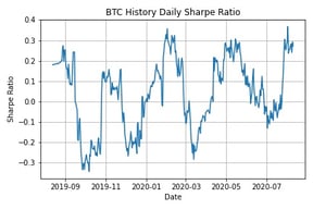
What you do next with the data is up to you, but let’s dive a little deeper and start looking at the Sharpe ratios of other assets as well for context.

Traditional Assets Sharpe Ratio

We are going to look at the Sharpe ratios of a couple of the most common assets, namely the S&P 500, Apple, the Vanguard Bond index, and gold futures. For this part we need outside data sources, so I used the pandas datareader package as an easy and free way to get daily historical stock data. This package gives you data from Yahoo! Finance. The code for this portion was adapted from the Udemy course Algorithmic Trading & Quantitative Analysis using Python by Mayank Rasu. We can simply get daily OHLCV data with pandas datareader:

From here we calculate the Sharpe ratio using these helpful functions. These assume that the assets are only traded 252 times a year, which is the case for stocks on the NYSE for example but not all assets. Cryptocurrency for example can be traded at any time, so for those we would use 365 instead of 252.

Once we calculate the Sharpe ratios for each asset, we can plot the results along with the bitcoin Sharpe ratio.

historical sharpe ratios

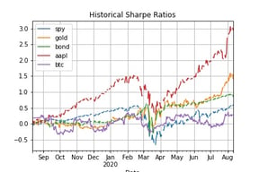
Notice how spotty the data from pandas_datareader is. Unfortunately this is to be expected from most free and easily available data sources, especially for financial data. This is fine because this is just for demonstration purposes, but you would want to find a much better data source (like Amberdata) if you were doing this for your investments.

It looks like bitcoin is the odd one out here. We can see that gold, Apple, US bonds, and a large cap index — the S&P 500 — all followed together in the past year, likely as a reaction to the global pandemic. Of course Apple performed particularly well, but surprisingly gold and bonds have done much better than the market index since about February. What else we notice though is that bitcoin does not seem to move with the other assets, and seems to be much more uncorrelated to stocks than even gold — the traditional hedge against equity. Let’s push this a little bit further and take a look at the Sharpe ratios of just digital assets.

Digital Assets Sharpe Ratio

Let’s take a look at the historical sharpe ratios of just digital assets this time. I selected six for us to focus on: bitcoin, ethereum, chainLink (LINK), Stellar (XLM), bitcoin cash (BCH), and bitcoin satoshi vision (BSV). If you are interested in learning more about these assets I suggest you do some digging, but I just decided to select a couple from the top 10 tokens by market cap at the time of writing. We can easily get the data from those five and plot the result. You may have your own method, but here is how I did it:

If we join the results and plot, we can see that the digital assets tend to move together.

digital asset sharpe ratios

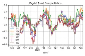
These digit assets returns seem to be highly correlated. We can look at the correlation between the coins and confirm that in general, this is indeed the case.

square box

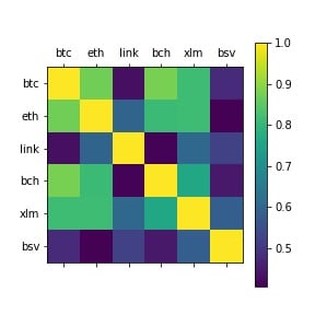
However, LINK — or ChainLink Token — is correlated with bitcoin by less than 0.5. We can confirm this by looking at the coins most and least correlated with our benchmark: bitcoin.

Most similar returns to BTC: BCH
	Correlation: 0.8787211313283082

Least similar returns to BTC: LINK
	Correlation: 0.43102576098847994

A correlation of 0.43 is pretty low for securities, so ChainLink may be an interesting way to add diversification into a portfolio for digital assets. We also notice that bitcoin cash’s returns are unsurprisingly the most correlated to bitcoin. This will change periodically, but is a good thing to keep in mind when investing in digital assets.

Let There Be Returns

In conclusion, we went over some key background on the Sharpe ratio and its lesser-known cousin, the Information ratio and why they are important. We took a quick look at how to use Python to calculate the historical daily Sharpe ratio for bitcoin, as well as several other assets across different classes. I hope this primer on the Sharpe ratio helps you to understand that there is more to investment than just pure returns, and you learned something new about manipulating financial data in Python. Stay tuned for more blog posts where we dig through the hairy mess that is blockchain data.

The code for this blog post is available here.