Share this blog:
Bitcoin has outperformed most assets and many believe that the trend will continue for the foreseeable future. However, simply buying and holding digital assets may expose you to more volatility than you may be comfortable with. What if you could go back in history and buy Bitcoin when it was trading at a discount and likely oversold? Could you replicate Bitcoin’s returns to date for less risk?
Backtesting trading strategies allow us to test our hypothesis and quantify historical performance. This is the third post in our series “Digital Assets for fun and profits”. In this post, we are going to scope and develop a hypothetical trading strategy, backtest it using Backtrader, quantify our results, and create some Alpha. For the record, this is an educational post on how to backtest a cryptocurrency trading strategy and not investment advice.
I work at Amberdata so we are going to use our APIs. You will need an API key to code along with us during this series of posts. To get started sign up for the OnDemand plan. Next, you will need to setup Backtrader a python framework for backtesting and trading. You can also download the trading strategy code here if you want to follow along.
Below is the idea we will backtest:
- What if we had bought Bitcoin when it traded at a discount to the stock-to-flow modeled value developed by PlanB.
2. We would want to buy the reversals when the market was oversold. We will use MACD, a trend-following momentum indicator to identify these reversal opportunities. We will enter our positions when the trend is still down, yet, the MACD Signal crosses above zero indicating reversal momentum.
3. Once in the trade, we will place a percent trailing stop with enough breathing room to stay in the trend as long as possible.
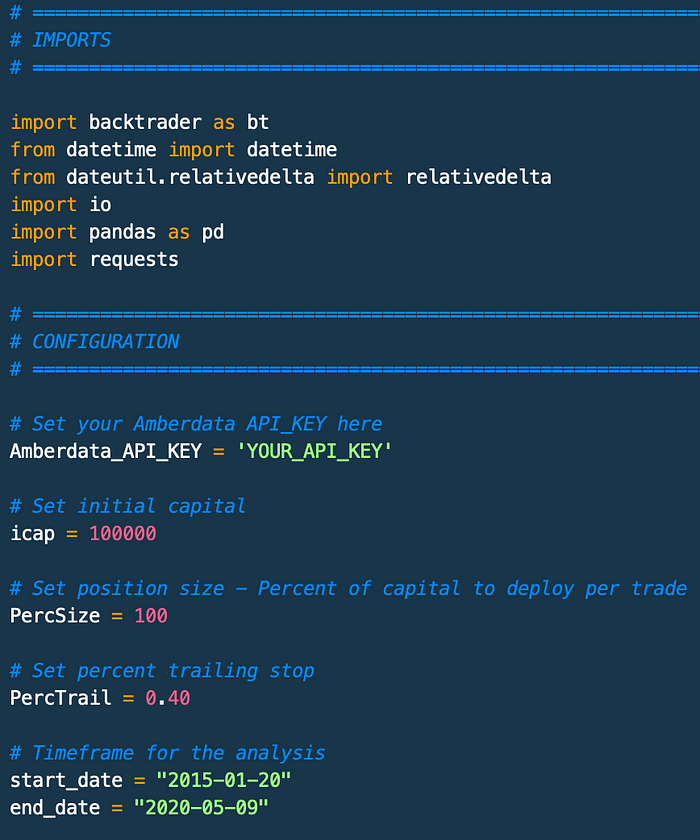
Let's start coding up our strategy and see how it performs. We need to import backtrader, pandas, and requests so we download, prepare, and load our data into Backtrader where we will quantify our trading algorithms performance.
We pulled our variables for your API_KEY, Initial trading capital, Percent position size, Trailing Stop Percent, and start and end dates to the top for easy configuration.
Now we will pull the historical market and metrics data we need to backtest our strategy from Amberdata. We are going to use market data (Open, High, Low, Close, and Volume) and Stock-to-flow model valuation end-points. Think of on-chain data and metrics like fundamental data in traditional financial markets. What is really cool here is we are providing you with the tools to test any combination of metrics, on-chain, and market data derived strategies for any digital assets. After this post, if you can think it, you should be able to code it up and backtest your strategy.

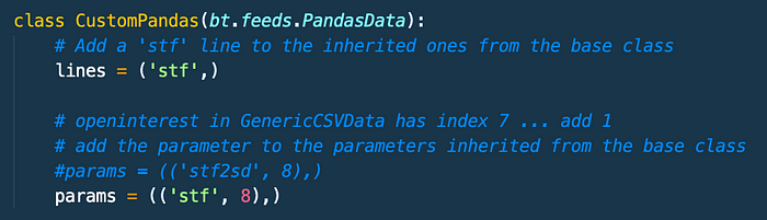
Next, we will define a class so we can append non-price data to Backtrader. Backtrader uses a concept called lines to pipe data into the backtesting engine. The expected format is Timestamp, Open, High, Low, Close, Volume, Open Intrest. We append our stock to flow ‘stf’ model data into an 8th position so we can reference it from within the strategy.
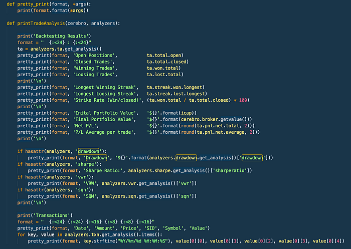
Next, we will set up our backtrader analyzers to help us instrument our strategy and quantify the results of our research. I looked at and compared the systems Sharpe Ratio, VRW, and SQN when iterating against variations of our strategy.
The strategy is pretty simple… If the MACD Signal (9-period EMA) crosses over the zero-line, while the trend is still down as measured by a 10-period/30-period SMA cross-over being negative this could indicate a reversal.
But we still need to know that Bitcoin is undervalued as compared to the stock-to-flow model valuation. So we will also require that the close of the last bar is also less than the valuation modeled by the stock-to-flow model.
The Backtrader documentation had a good MACD example strategy that helped us hit the ground running. We replaced the ATR Stop with a percent trailing stop and added additional valuation entry criteria using stock-to-flow.

In summary, the strategy is as follows:
- MACD Signal > 0.0
- SMAdir < 0.0
- Close < Stock-to-flow modeled value
- Buy
- Set a Percent Trailing Stop to take us out of the market if there is a violent pull back.
When you start to build your own strategy you can use this code as a template that pulls in your data, instruments your strategy, position sizes, and generates a report. Simply insert your strategy into the Strategy Class.
Next, we need to create an instance of Cerebro, some observers, set the investment capital to run our strategy as defined upfront in the icap variable.
We have also leveraged the Cerebro’s position sizer which is really awesome, enabling you to allocate your position size based upon a percentage of your total account value.
For simplicity, we have used 100% of capital allocated to this strategy though in the real-world it would likely a single-digit percentage of your account. (Not financial advice).
We then Add the strategy to Cerebro, feed the market, and metrics data into a data frame and then...

We can then run the strategy… drum roll.

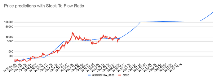
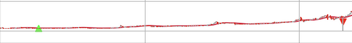
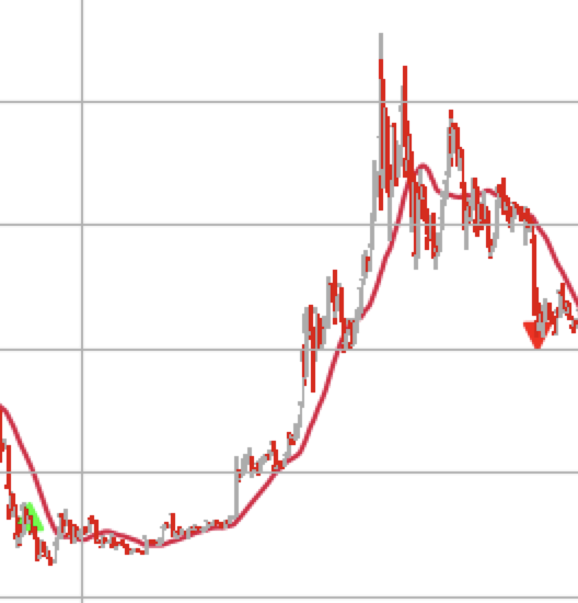
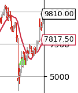
You can see from the chart above that we successfully bought the dips where Bitcoin was valued less than Stock-to-flow. You can see below, we have charted the price time-series and overlayed the STF modeled value.

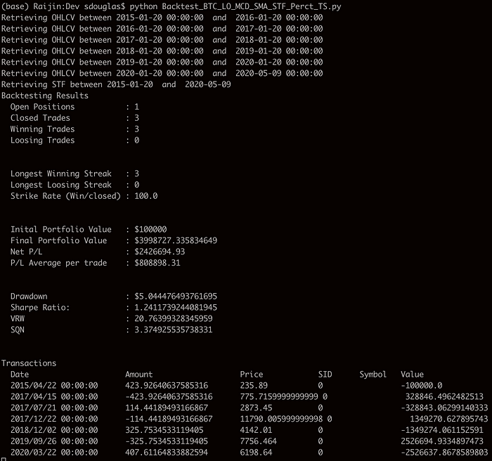
Between 1–20–2015 and 5–10–2020 we invested $100,000 and only did 4 trades three of which we closed profitably. With our final portfolio value being $3,998,727. We had a 100% win rate with no more than a 40% drawdown in any trade.
1. Profit: $328,846
2. Profit: $1,349,270

3. Profit: $2,526,694
4. Open Still …
The system produced these returns along with some impressive metrics. It would have been nice to have had a few more trades however, our strategy really needed Bitcoin to be undervalued, in a downtrend, and to catch a momentum-based reversal coming off the lows. So the stars really need to align. When the strategy fired the buy signal, bitcoin was undervalued, oversold, and starting to turn up which is pretty exciting. Once long, we held as long as possible until we were stopped out with our trailing stop.
The results:
SQN: 3.374
VRW: 20.763
Sharpe Ratio: 1.241
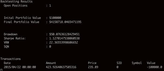
So the obvious next question we should ask ourselves is how does this compare to simply buying and holding? Buying and holding you would have made you an additional $159,991 however you also have had to endure an 85% drawdown living through a plummet from an all-time high of $20k down to ~$3k. Would you have held-on?
The strategy we built has you getting stopped out rather than living through that. As such when we compare Sharp Ratios between the systems we show a slightly better risk-adjusted return of 1.241 vs 1.127 versus just HODLing.

In summary, you have learned to build, backtest, and quantify your Cryptocurrency trading strategy using the Amberdata API for fundamental and market data using Backtrader.
We invite you to sign up for the OnDemand plan, setup Backtrader and start using python backtesting and trading ideas. You can download the strategy code here.
Here is a link to the Stock-to-flow model end-point. Can you outperform this simple strategy?